Linear Regression
Fit a line through two variables to expose relationships and highlight influential outliers.
Fit a regression line to the predictor and response, then inspect the residuals to find observations the model fails to explain. Large residuals or high leverage points reveal influential outliers that can distort the slope and deserve follow-up.
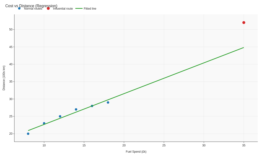
Image source: generate_visuals.py
Code examples
Building a quick regression
import pandas as pd
from sklearn.linear_model import LinearRegression

# Simple spend versus sales dataset
data = pd.DataFrame(
    {
        'Spend': [10, 12, 13, 15, 30],
        'Sales': [22, 24, 25, 27, 45],
    }
)

# Fit the regression model
model = LinearRegression().fit(data[['Spend']], data['Sales'])

# Generate predictions and residuals for diagnostics
data['Predicted'] = model.predict(data[['Spend']])
data['Residual'] = data['Sales'] - data['Predicted']
print(data)
' Regression coefficients and predictions
=LINEST($B$2:$B$6,$A$2:$A$6,TRUE,TRUE)
=FORECAST.LINEAR(A2,$B$2:$B$6,$A$2:$A$6)

' Residuals to assess model fit
=Actual - Predicted
// Slope of the regression line using covariance / variance
Reg Slope =
    VAR Numerator =
        SUMX(
            'Data',
            ('Data'[Spend] - AVERAGE('Data'[Spend]))
                * ('Data'[Sales] - AVERAGE('Data'[Sales]))
        )
    VAR Denominator =
        SUMX(
            'Data',
            ('Data'[Spend] - AVERAGE('Data'[Spend]))^2
        )
    RETURN
        DIVIDE(Numerator, Denominator)

// Intercept for the regression line
Reg Intercept =
    AVERAGE('Data'[Sales]) - [Reg Slope] * AVERAGE('Data'[Spend])

// Predicted sales using the regression components
Reg Predicted = [Reg Intercept] + [Reg Slope] * AVERAGE('Data'[Spend])

// Residual to highlight outliers from the line
Reg Residual = AVERAGE('Data'[Sales]) - [Reg Predicted]
Key takeaways
- Regression helps you quantify relationships and spot influential points.
- Always inspect residuals; they reveal whether the model fits evenly across the range.
- Explain assumptions (linearity, no hidden factors) before presenting results.